Seemingly the field of reliability growth modelling (cf. ch. 3 "Software Reliability Modeling Survey" in Lyu's book from 1996) is facing the same basic, i. e. philosophical, problems as the so called historicism. According to Popper long-term prophecies cannot be applied to social systems we are all caught in. And "it is wise to combat the most urgent and real social evils one by one, here and now" (Popper, 1963).
From the very beginning, when I came across the reliability growth models for the first time I felt compelled to apply Popper's rules of falsifiability, corroboration, and simplicity to them.
What follows is an assessment of reliability growth models in respect to their prognostic strength and their ability of supporting the learning from errors. This is done under the light of Popper's criteria and by means of statistical measurement. The questions to be answered are: What is the predictive strength of the highly sophisticated reliability growth models? Is the effort worth the result, or is it even misleading? What can be learned from reliability growth models? Which methods - if any - are better suited for the software engineer's task.
Classical reliability theory is well founded: Much effort has been spent toward the collection, classification, and analysis of failure rate data of hardware components (Shooman, 1990). Under certain conditions the life time (time to first failure) of hardware components can be conceived to be an exponentially distributed random variable. The reliability function R(t) of an object (component or a system) is defined to be the probability that the time to failure is greater than t. With a constant failure rate l this function is given by R(t) = ![]() .
.
Now let a program be given containing some errors. Under the presupposition of constant operational profile a constant failure rate l can be assumed. From this the reliability function looks like the one given above for hardware failures.
There is one crucial difference: a failure is now conceived to be a volatile occurrence and does not result in a permanent defect. The defect was there from the beginning.
We are assuming some effort of fault removal. From this follows a new and unknown failure rate. By this the assessment of failure rates by past experience seems to be impossible from the beginning.
What can be done? We can try to pull us out of these difficulties by our own boot-straps. Every so called Reliability Growth Model (RGM) is based on specific assumptions concerning the change of failure rates through fault removal.
Such an assumption is the core of the respective model. It is meant to represent the empirical content of the RGM.
One of the typical assumptions is the one of the Jelinski-Moranda model (Lyu, 1996): Through fault removal the failure rate will be reduced by a certain value which is constant for all faults.
The central question is, whether such assumptions can be corroborated.
There is a method known from the weather forecast, the "trivial forecast": Tomorrow the weather will be the same as today. This trivial forecast has some predictive accuracy. I wondered whether a trivial reliability growth model could compare well with the highly sophisticated models under the light of the statistical criteria.
The Trivial Reliability Prediction (TRP) model to be introduced does not assume any reliability growth. It is applicable to systems with a constan failure rate. Under this assumption the times between failures of the past can be used for assessing the mean time between failures, or its reciprocal, the failure rate: The mean value of the last - say five, or ten - execution times between successive failures is taken as an estimate of the mean time between failures.
The TRP is a fairly simple model that is commonplace in hardware reliability. It possesses all the ingredients any widely acceptable theory should possess:
Why do we put the TRP - knowing that it is based on the assumption of unaltered reliability - into competition with the more elaborated models assuming reliability growth? It is because we don't know how the failure rate changes after fault removal. The system could change much - to the better or to the worse. But very often it seems to be justified assuming no change at all, because the fault removal has only marginal effects on system reliability.
Reliability growth models are meant to predict the future behaviour of software on the basis of past experience. Past experience in this context is based on historical data; the predictions cannot be corroborated by means of experiments.
Knowledge is synthetic (or empirical) insofar as certain assumptions are involved which are not valid a priori and which are to be corroborated through experience. It is analytic in those parts which are solely based on logical deductions and mathematics. The criteria Popper (1980) puts on the synthetic or empirical content of prediction methods - the predictive strength of the methods - are:
With respect to objectivity the RGM are not worse than other prediction methods. But in my opinion all the other of Popper's criteria are missed by RGMs.
Reliability growth models cannot be falsified in the sense of Popper's criterion of falsifiability. This is mainly due to the fact that there is an abundance of models and parameters such that it is nearly impossible not to find a model fitting with some given experimental or field data.
Thus the models don't fulfil the criterion of simplicity. In this context "simple" doesn't mean "easily understandable". A (simple) straight line fitting with some points in the plane is more convincing and possesses more empirical power than the fact that the points may be approximated by some higher order curve (not simple).
Consequently these models cannot be corroborated (in Popper's sense). In all demonstrations of the models I know so far, the selection of a model and its fitting to the data is done in retrospect. I don't know any falsifiable and non-trivial prediction scheme for software reliability on the basis of these models.
The above mentioned philosophical criterea are lacking the touch of serious engineering. Therefore I looked for and found some engineering-like criteria for the predictive accuracy of reliability growth models in a contribution by Bev Littlewood to the Software Reliability Handbook (1990):
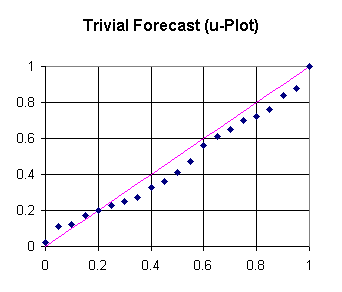
The u-plot of the TRP on the basis of Musa's data (taken from the above mentioned Software Reliability Handbook, p. 139) is given in fig. 1. The maximum deviation of the u-plot from the uniform distribution (the diagonal line) is taken as an indication of predictive inaccuracy. The deviation amounts to 0.090.
This figure compares well with those obtained by the models which have been investigated by Littlewood: Jelinski-Moranda (0.1874), Littlewood-Verrall (0.1437), Littlewood Nonhomogeneous Poisson Process (0.0805).

Fig. 1 u-plot of the trivial reliability prediction
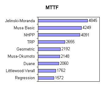
Fig. 2 shows some estimates from some of the best known reliability growth models together with the estimate given by the trivial reliability prediction. The predictions are covering a wide range. The trivial reliability prediction - the only prediction not assuming reliability growth - lies somewhere in between the extreme values.
All estimates are accompanied by a certain confidence interval. In the case of the TRP and under the precondition of an approximately constant failure rate we can be 90 % sure that the mean time to the next failure (MTTF) is not smaller than 1487 and not greater than 6638. This interval cannot be reduced considerably by taking into consideration a larger number of recently observed times between failures. The confidence intervals of the other methods may be a bit smaller - but certainly not small enough for the disqualification of the TRP.
The competitiveness of the trivial forecast can be attributed to the fact that there will be a tendency for the large faults (measured by their probability of occurrence) to show themselves earlier than the small ones. At the end of the debugging process supposedly many small faults are remaining such that each fault removal will not change very much, indeed.
The preceding paragraph suggests that the TRP may possibly have some empirical content: The model is simple and, because its goal is so modest, it could possibly be corroborated for software with a lot of small faults, i. e. for unreliable software in a later phase of debugging.

Fig. 2 Estimates of some reliability growth models and the TRP
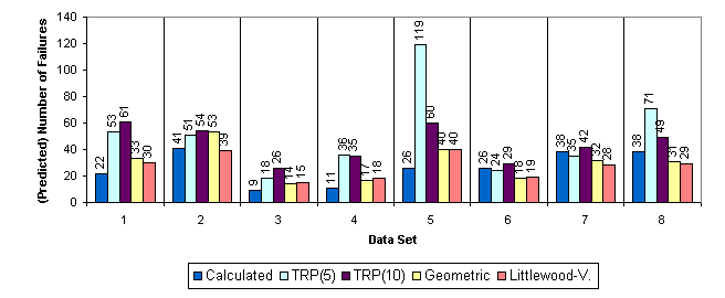
For further investigation of the competitiveness of the TRP a simple experiment had been designed. Eight data sets of failure data were constructed by means of a simulation using the Jelinski-Moranda (JM) and the Geometric (G) reliability growth model. These data covered two time periods, each extending over 10000 time units. The failure rates l 1, l 2, l 3, ... are assumed to decrease according to l i+1 = l i - F . (Jelinski-Moranda model) or l i+1 = r l i (Geometric model) with constants F or r, respectively. For convenience we denote by N = l 1/F the number of failures in the Program (JM model) and we set MTTF1 = 1/l 1. The generating models of the eight data sets are shown in table 1.
The set up of the experiment was such, that the reliability assessment had to be done on the data from the first time period. The prediction should give an estimate of the number of failures during the second time period. Fig. 3 shows the result of the experiment. For all data sets the TRP(10) - the trivial reliability prediction on the basis of ten recently observed times between failures - compares favourably with the assessment by means of the Geometric or the Littlewood-Verall model.
These two models (Geometric and Littlewood-Verall) were selected from a greater collection of reliability growth models because they produced the best predictions. It should be noticed that the data sets 3 through 8 were generated by means of the geometric model; therefore it is no wonder that this model performs especially well.
Table 1 Parameters of the test data generating models
|
Data Set Number |
Model |
r |
N |
MTTF1 |
|
1 |
JM |
|
100 |
150 |
|
2 |
JM |
|
200 |
150 |
|
3 |
G |
0.95 |
|
150 |
|
4 |
G |
0.95 |
|
50 |
|
5 |
G |
0.98 |
|
100 |
|
6 |
G |
0.98 |
|
100 |
|
7 |
G |
0.99 |
|
120 |
|
8 |
G |
0.99 |
|
120 |
The method of testing a reliability growth model by means of simulated data can be criticized: One objection could be, that the reliability growth models are designed to predict the behaviour of real life processes but not the behaviour of some artificial models. Therefore these reliability growth models should be tested with data from some field experience and not with simulation data from models itself. This objection doesn't meet the point because of the following reasons.

Fig. 3 Results of an experiment
Even the proponents of reliability growth models don't trust in this theory to have any remarkable empirical content; they admit that nothing can be learned from reliability growth modelling about the commitment, the causes, and the avoidance of errors. This becomes clear from the following statement by Brocklehurst and Littlewood, found in Lyu's book (1996): "There is no universally acceptable model that can be trusted to give accurate results in all circumstances; users should not trust claims to the contrary. Worse, we cannot identify a priori for a particular data source the model of models, if any, that will give accurate results; we simply do not understand which factors influence model accuracy" (p. 156).
Management of software production should aim at error avoidance. The optimum learning from the errors of the past is a well established method of error avoidance, in engineering as well as in nature. But there is no contribution to this method from reliability growth modelling: "The models do not contain enough information to help explain the causes of a problem; moreover, they are not even able to tell us if there is a problem. The only thing the models will do is to make a trend explicit, but it is up to the user of the reliability growth models to interpret its meaning" (Miranda, 1998).
The conclusion to be drawn from these observations are: We should not spend much time in reliability growth modelling. Instead we should strive for error avoidance by applying methods which support our learning from errors. And there are a lot of methods offering exactly what we need:
Reliability Growths Models could make strong statements for weak and basically unaltered software or - at least - stable production processes. But the engineer should ask for strong software, and in the case of weak software he is forced to make revolutionary changes in the software production process. Reliability growth models are rendered completely worthless by such changes.
The engineer's effort seems to be badly allocated in the calculation of RGMs. He should better be involved in activities aiming at better software. These are the methods of fault-intolerance. (It should be kept in mind that fault tolerance does not belong to the engineer's virtues.)
We should not give up the principles of if-then-sciences and the principles of empiricism. This is because we want to learn something about our work and we want to predict the behaviour of our artefacts.
The best prediction method is the most simple one: The Trivial Reliability Prediction has some empirical content. It can be understood and safely applied by any engineer involved in reliability calculations.
Birolini, A.: Reliability Engineering. Theory and Practice. 3rd ed. Springer, Berlin, Heidelberg 1999
Dahl, O.-J.; Dijkstra, E. W.; Hoare, C. A. R.: Structured Programming. Academic Press, London 1972
Grams, T.: Denkfallen und Programmierfehler. Springer, Berlin, Heidelberg 1990
Gries, D.: The Science of Programming. Springer Heidelberg 1981
Kernighan, B. W.; Plauger, P. J.: The Elements of Programming Style. McGraw-Hill, New York 1978
Leveson, N.: Software Safety: Why, What, and How. Computing Surveys, 18 (1986) 2, 125-163
Littlewood, B.: Modelling Growth in Software Reliability. In: Software Reliability Handbook. Elsevier, London, New York 1990 (Edt: Paul Rook), pp. 137-153, 401-412
Lyu, M. R.: Handbook of Software reliability Engineering. IEEE Computer Society Press. McGraw-Hill, 1996
Meyer, B.: Object-oriented Software Construction. Prentice Hall, New York 1988
Miranda, E.: The use of reliability growth models in project management. ISSRE '98, 291-298
Myers, G. J.: The Art of Software Testing. Wiley, 1979
Parnas, D. L.: On the Criteria to Be Used in Decomposing Systems into Modules. Comm. ACM 5 (Dec. 1972) 12, 1053-1058
Popper, K. R.: Prediction and Prophecy in Social Sciences. In: Conjectures and Refutations. The Growth of Scientific Knowledge. Routledge, London 1963
Popper, K. R.: The Logic of Scientific Discovery. Unwin Hyman, London 1980
Shooman, M. L: Probabilistic Reliablilty: an Engineering Approach. Robert E. Krieger Publishing Company, Malabar, Florida 1990
Wirth, N.: Program development by stepwise refinement. Comm. ACM 14 (April 1971), 221-227
© Timm Grams, 10. August 1999